Untangle the concepts of explicability and generalization

1. Introduction

Concepts in data science can quickly become similar when we are not directly involved in the technical side of the field. Thus, concepts such as the generalizability of a model or its explainability can quickly be confused. The purpose of this article is to give the layman an overview of these concepts and to enumerate some strategies to validate the generalizability of a model regardless of whether it is explainable or not. Note that according to the context (business context, regulatory context, ethical context), it may be necessary to use models that allow us to understand the algorithmic process and the choices made by it, while in other cases, only the best prediction (on new data) is important. It is important to understand that an explainable model is not inevitably generalizable and that in some cases, a "black box" model can be more generalizable than an explainable model. A possible approach is always to test both explainable and black-box models, evaluate their generalizability and choose the final implemented solution based on the difference in performance between the two approaches.

2. Black-box models vs. explainable models

Before getting into the definition of a so-called "black-box" model and an explainable model, it is first important to understand the difference between interpretability and explainability of a model. Gilpin et al. [1] define the interpretability of a model as the understanding of what a model does. For example, if we take the case of a deep neural network that classifies images, we can visualize the places in the image where the model has defined and found patterns or representations in order to make its classification without, however, understanding precisely why the image has been classified in this fashion. As we can see in the figure on the right, the model constructs representations associated with faces in a more or less abstract way depending on the position in the deep network (the gray levels at level 1 allow to define rectilinear borders at level 2 which allow to define facial elements such as a nose, a mouth at level 3, etc.). Thus, if we can interpret at a certain level the functioning of such a model, it is however difficult, if not impossible, to explain in detail what the algorithm does to reach its conclusion. 

An explainable model is a model for which it is possible to define what is happening inside the algorithm and to put it in terms that are understandable by a human. Thus, an explainable model is interpretable, but the opposite is not necessarily true. From this point of view, a "black box" model is one for which one can generally interpret the result, but not explain it completely because of its complexity or the large number of variables present in the model. Consequently, some authors such as Rudin [2] propose to use only explainable models to motivate decisions that have an important impact on a company or society.

3. Breakdown of interpretability

In his book Interpretable Machine Learning, unlike Gilpin [1], Molnar [3] does not make a distinction between interpretability and explainability and uses these terms interchangeably. On the other hand, Mortar breaks down the concept of interpretability into 5 categories. The questions he attempts to answer and the concepts are as follows:

Transparency of the algorithm: How does the algorithm create the model?

Global interpretability of the model: How does the trained model make predictions?

Global interpretability of the model at a modular level: How do different parts of the model affect predictions?

Local interpretability for a prediction: Why did the model make a certain prediction for a given observation?

Local interpretability for a group of predictions: Why did the model make specific predictions for a group of observations?

Finally, the concept of XAI ("eXplainable Artificial Intelligence") has been developed. It combines the aspects of transparency, interpretability and applicability [5] . We note that different methods exist to evaluate the interpretability of a model and we let the reader's curiosity lead him to go and dig for more information.

4. The link between the explainability and the performance of a model

While it is sometimes required to explain how and why the model makes its predictions, it is always desirable to have an acceptable level of performance. Some authors have illustrated (cf. fig *below*) the relationship between the interpretability of a family of algorithms and the accuracy of the predictions it generates. Thus, it is essential to evaluate the characteristics and needs of one's own project in order to make the appropriate choice.

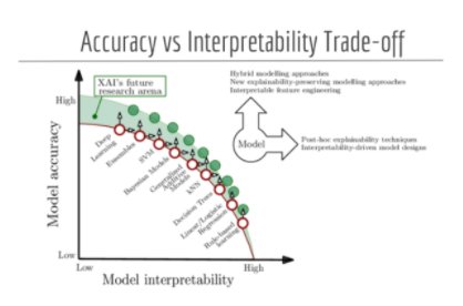
Source: DPhi Advanced ML Bootcamp — Explainable AI - DPhi Tech, Explainable AI Course, https://dphi.tech/lms/learn/explainable-ai/563

It should be noted that the previous figure is very general and that depending on the context, a model that is lower on the accuracy axis can be of the same level of performance or even better than models located further north on the axis. In order to compare them, a good practice is to have a so-called "baseline" model, which is often less complex.

Apart from the concepts of interpretability, explainability and accuracy, it is crucial to develop generalizable models, i.e. to be able to be effective on new observations that the algorithm will never have seen.

5. Model generalization

The importance attributed to the generalization capability of a model is due to the fact that we want the model to perform well on observations that it has never seen before. To do this, different strategies or techniques exist in order to avoid over- or under-learning. If you are unfamiliar with these concepts, the image below is a good representation. We want the model to fit our data well, i.e. to capture the "signal" it contains as well as possible, but to avoid fitting to the noise. In the latter case, this means that the model would have learned a certain structure in the data that is only applicable to the sample it was given during training and is therefore not generalizable. 

To characterize this, we can use the generalization error, i.e. the error obtained on a test sample different from the training sample, as shown in the graph in Figure 4. This generalization error decreases with the increase in the model's capability (we are then in the under-learning phase) until a given optimum is reached. After this optimum, the increase in capability has a negative effect on the generalization error (we are then in the overlearning phase). But what is the capability of a model? The capability of a model can be defined by its complexity or by its ability to adapt to a large variety of functions[3]. A linear model will therefore have a lower capability than a quadratic model, for example. Thus, the analyst must find a middle ground in order to limit the under- or over-learning of the model.

Différentes méthodes existent dans le but de sélectionner la bonne capacité de modèle et ainsi de réduire l’erreur de généralisation. Certaines sont présentées ci-dessous. 

A) Likelihood based indicators

In order to choose a probabilistic model that reproduces the distribution of the data, certain indicators such as the AIC (Akaike Information Criterion) and the BIC (Bayesian Information Criterion) can be used to avoid overfitting the data. Indeed, these indicators, which are calculated directly on the training sample, penalize the addition of extra parameters in the model. They thus make it possible to make a compromise between the quality of the adjustment and the complexity of the model. If these metrics allow us to choose among several models the one that is likely to have the best generalization capability, they do not however allow us to directly access the value of the generalization error. One could compare these metrics to a compass; they allow us to know where to go, but without ever having an idea of the distance covered or what remains to be done before arriving at the destination.

B) Sample separation based methods

Dividing the sample data is one of the common techniques to 1) maximize the generalizability of the models and 2) to have an evaluation of this generalizability. Data sampling is thus one of the most important parts of developing a predictive model. Essentially, it is important to analyze the data and choose the appropriate sampling method while taking into account certain constraints such as sample size or data balancing for example.

i) Training, validation and testing sample

Before starting to train an algorithm/model, it is possible to divide its dataset into several samples when the dataset is large. Why? In order to have data that have never been seen by the model to be able to correctly estimate its generalization ability. Thus, we usually generate three data sets. A training sample on which the algorithm is trained. A validation sample distinct from the training sample on which we compare the performance of several models. Indeed, it is not uncommon to train several different models in order to find the best model. Once the best model is defined, we select the one with the lowest error on the validation sample and re-evaluate its performance on the test sample. 

ii) Cross-validation

When dealing with small samples, the division of the sample into training, validation and test samples can be problematic. In such cases, the use of the cross-validation technique is recommended. As shown in figure X above, this method consists in dividing our training sample in order to have k different samples (often 5 or 10) in order to use different data during the training and validation of the model. Thus, using the example in Figure X, for a 5-fold cross-validation, the model will be trained 5 times. At each iteration, the data that will be used to fit the model will be different (the data in pink) and its performance will be evaluated on the rest of the data (in blue). By obtaining a performance metric(s) for each of the k training and validation runs, it is possible to obtain an estimate of the generalization error while saving a validation sample. When the parameters of the best model have been identified, we can then re-train our model on the entire training data to obtain the final model.

Finally, other sampling techniques exist and can be better adapted to the dataset used in the modeling. Indeed, according to the balance of the dataset, it is possible to use oversampling techniques (Random Oversampling, SMOTE, ADASYN, Data augmentation) or undersampling (Random Undersampling, Tomek Links, Near-Miss) to allow the model to better learn from the rarer cases present in the dataset.

C) Regularisation

Regularization is a complementary technique to the two previous techniques. Schematically, its principle is to use a model which is too complex and which should normally lead to overlearning, but to add artifices to adjust the effective capability of the model. Among the regularization techniques, two methods are popular: the L1 and L2 penalty methods. Without going into the theory and the complexity of these methods, they allow the penalization (i.e. the reduction) of the model coefficients. Thus, to take the example of figure X above, it would be possible to use a polynomial model of degree 3, 4 or 5 for example, but to limit the coefficients of the model to small values. To do this, a parameter (often called alpha) is added to calibrate the intensity of the regularization. This parameter can be adjusted in order to reach better performances while decreasing overlearning (this can be done in cross-validation!). These methods can be applied on simpler models such as linear regression as well as on neural networks which are more complex.

Other regularization methods are specific to certain families of models just like the "dropout" is for neural networks.  Indeed, this technique allows to reduce the complexity of the network by ignoring a proportion of the data during the training and thus allowing the model to be more generalizable by reducing the over-training.

6. Conclusion

These concepts may seem daunting, but it is important to remember that the use of certain predictive models must be tailored to the needs one is trying to meet. The first criterion to consider is whether it is necessary to be able to interpret and understand the predictions of the trained model. If this is the case, it is preferable to limit oneself to certain families of models that are said to be explainable. Regardless of the choice of explicable or non-explainable model, the chosen model must still be generalizable so that its performance is acceptable on unknown data. To do this, certain techniques can be used to ensure that even "black box" models can be generalized. 

[1] Gilpin, L. H., Bau, D., Yuan, B. Z., Bajwa, A., Specter, M., & Kagal, L. (2018, October). Explaining explanations: An overview of interpretability of machine learning. In 2018 IEEE 5th International Conference on data science and advanced analytics (DSAA) (pp. 80-89). IEEE.

[2] Rudin, C. (2019). Stop explaining black box machine learning models for high stakes decisions and use interpretable models instead. Nature Machine Intelligence, 1(5), 206-215.

[3] Molnar, C. (2020). Interpretable machine learning. Lulu. com.

[4] Goodfellow, I., Bengio, Y., & Courville, A. (2016). Deep learning. MIT press. p.115

[5] Wikipedia, https://en.wikipedia.org/wiki/Explainable_artificial_intelligence, as seenn on septembre 21, 2021.