Insurance data representation with Bayesian networks

7 minutes

Understanding one's dataset can often be a complex task. Graphical probabilistic models (PGMs) such as Bayesian networks add a level of understanding to the field of study by graphically representing the structure of variables.

PGMs use graphs to represent a multi-dimensional space and allow the encoding of relationships between variables with the help of probabilistic models.

To illustrate its use, we will browse through a data set of automobile insurance customer information (20,000 observations, 27 variables). Here is an overview of some of the variables (all categorical):

An example of a Bayesian network structure for this example:

[image library R: bnlearn]

The learning task of a Bayesian network consists of three subtasks: 

1. Structural learning, i.e. the identification of the network topology; 

2. Parametric learning, i.e. the estimation of numerical parameters (conditional probability distributions - CDP) for a given network. 

3. Inference queries can thus be made using the resulting graph, for example by taking a portion of a person's variables in order to evaluate the distributions of other variables of interest.

The purpose of the paper is to present some of the methods of the first two steps for the automobile insurance data set. For a better understanding, let's define some concepts.

1. Some concepts 

Let's start by describing some concepts applied to our context.

Random variables: The explanatory variables.

Conditional Probability: Let's take the example of automobile insurance data. The probability that a person will have an accident knowing that they have had an accident is expressed as follows: 

Probability (Accident | already had accidents) 

Independence and dependency: When the event of having an accident is not influenced by having had an accident in the past, these two variables are said to be independent, otherwise dependent. 

The set of variables X1, X2...Xn are considered independent if

Conditional probability distribution: When variables are categorical, a conditional probability table (CDP) is used to represent the conditional probabilities.

The conditional probability distribution of "Accident" given "previous_accident" is the probability distribution of Accident when the value of "previous_accident" is known.

Graph: In most graphical representations, nodes correspond to random variables, and arcs correspond to the probabilistic interactions between them. [4]

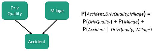
The purpose of the graph is to capture how the joint distributions on all variables are to be decomposed into a product of factors, each dependent only on a subset of the variables. 

An example of a simple Bayesian graph (also called oriented graph) :

Bayesian network: Bayesian networks are graphs where nodes represent domain variables, and arcs represent causal relationships between variables [5]. This gives a compact representation of conditional probability distributions (CDP).

DAG (Directed Acyclic Graphs): In this article, we will focus only on directed graph models, i.e. Bayesian models. These models have the particularity of being represented by acyclic directed graphs (DAG), where we can informally interpret that the arc X1→ X2 indicates that X1 causes X2.

2. Step 1: Learning the network structure

The task is to find the most representative graph of the data. The methods to solve this problem are based on optimization methods. There are different approaches to learning network structure : 

• Les méthodes basés sur les scores (Likelihood, BIC, BDeu)

• Les méthodes basés sur les contraintes

• Les méthodes hybrides qui combinent les deux types d’approches

2.1 Scores - based methods

In order to assess the likelihood of the graph in relation to the data, the methods use a score. The differences between the methods lie in the type of score and the type of steps to optimize this score. This can be summarized in two steps: 

• A scoring function, which determines the likelihood between the data and the graph;

• An optimization problem, to maximize this same score. 

Research by the Hill-climbing method

It is an optimization method that allows finding a local optimum among a set of configurations. The algorithm starts from an unconnected DAG and manipulates arcs to a local minimum. This method is similar to the gradient descent method but adapted to discrete data, where the gradient cannot be defined.

Keeping 4 variables from the initial dataset, we obtain the following graph :

2.2 Constraint method

This approach is based on the creation of a list of constraints, which represents the links between the variables to be included in the final graph. This is first done by identifying the independences in the dataset using hypothesis testing. Then a DAG is constructed according to its independences. 

The level of confidence for the independence tests must be provided to the function. 

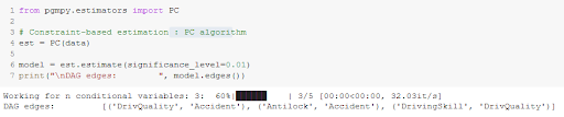
We get the same graph as the previous method :

If the graph is sparse (i.e. few nodes are adjacent to many other nodes), the PC algorithm is efficient [7].

2.3 Hybrid method

There are also hybrid methods that combine the two types of approaches, starting with learning a non-oriented graph with constraint-based methods and orienting the links with a scoring method. 

The MmhcEstimator.estimate() method of the python package pgmpy performs both steps and directly estimates a Bayesian model, but the method is not stable yet. Other libraries are more complete on R, including Bnlearn.

The methods of the pgmpy package return a list of arcs without graph visualization, but this can be done with some visualization efforts using NetworkX for example.

3. Step 2: Learning the parameters

The task is to estimate the values of conditional probability distributions (CPD). There are several methods for estimating them including : 

• Maximum Likelihood Estimate (Maximum Likelihood Estimate)

• Bayesian Estimate

Maximum Likelihood Estimation

From the graph constructed in the previous step and from the data, we can learn the joint probabilities at each of the nodes, according to its parent nodes.

Let's start by creating a Bayesian model, which contains methods for learning the parameters.

One way to express joint probability distributions (JDPs) is to use the relative frequencies for which the variables were observed. This is because the simplest distribution for discrete data is the Bernoulli distribution, and the maximum likelihood for a Bernoulli is the mean of the number of times the event was observed. This method is called the Maximum Likelihood Method (MLM).

We obtain the following conditional probability tables :

The disadvantage of the Maximum Likelihood approach is that the estimate of the parameter (in this case, the mean), does not indicate confidence in that parameter. If the event is never observed the value will be 0.

Bayesian Estimation

A more accurate estimate can be obtained with Bayesian estimators, which take into account the space of the structures and the possible parameters to find the structure of the graph that best reflects the data. Score functions such as the BDeu use different a priori (structures and parameters) and allow a more realistic estimation.

CDPs obtained by MLE (left) and Bayesian Estimator (right)

It can be seen that the probability that a person has expert level driving skills (variable Driving skill = Expert), does not have a 100% probability of having a normal driving quality (Driving Quality = Normal), but rather a 60% probability. Indeed, this seems to be more realistic.

4. Things to keep

Bayesian models can be useful for : 

• Obtain a global and compact vision of the dependency relationships between the variables with the network structure. This can be done from knowledge about the data or directly from the data alone. 

• Validate our understanding of the independence relationships between variables. Once the structure is learned, dependencies can be validated and added to a constraint learning approach. 

• Perform a query on the resulting graph to obtain the conditional probability distribution for a variable.

  5. Example of other applications :

Simplification of client forms in life or health insurance, or any other field containing the concept of risk. Forms can be optimized by understanding the influence of certain answers, and by proposing targeted questions only when they are associated with a certain risk. Simplifications can thus be supported by probabilistic models and an understanding of data structure.

This is a different approach to factor analysis where the goal is usually to cluster and identify latent factors, compared to Bayesian networks which can provide a structure of existing variables. The other difference is that Bayesian networks can also provide an estimate of the distributions of their variables to justify simplification decisions for example.

Deduce information about a person from partially completed profiles. 

References 

[1] Image https://bookdown.org/MathiasHarrer/Doing_Meta_Analysis_in_R/_figs/networks.jpg 

[2] Insurance evaluation network (synthetic) data set. https://www.bnlearn.com/documentation/man/insurance.html 

3] image R library: bnlearn https://www.bnlearn.com/bnrepository/discrete-medium.html#insurance 

[4] Probabilistic Graphical Models: Principles and Techniques / Daphne Koller and Nir Friedman. https://list01.bio.ens.psl.eu/wws/d_read/machine_learning/BayesianNetworks/koller.pdf 

[5] (2011) Bayesian Network. In: Sammut C., Webb G.I. (eds) Encyclopedia of Machine Learning. Springer, Boston, MA. https://doi.org/10.1007/978-0-387-30164-8_65 

[6] Robinson R.W. (1977) Counting unlabeled acyclic digraphs. In: Little C.H.C. (eds) Combinatorial Mathematics V. Lecture Notes in Mathematics, vol 622. Springer, Berlin, Heidelberg. https://doi.org/10.1007/BFb0069178 

[7] Richard E. Neapolitan. Learning Bayesian Networks. Publisher: Prentice Hall, Year: 2003

Notebook of examples with the PGMpy library : https://github.com/pgmpy/pgmpy_notebook/blob/master/notebooks/9.%20Learning%20Bayesian%20Networks%20from%20Data.ipynb

---